(last updated: March 14th, 2021)
Introduction to defSim
This short tutorial explains the basic functionality of defSim. First, we show the two main functions that create a single simulation run or a full experiment as a set of simulation runs with different parameter settings. The arguments are used to call a number of modules that are already implemented in defSim and can be combined to create a unique experiment. Then, we show the more modular use of defSim, where the modules are used independently or modified and fed back into the Simulation or Experiment classes.
1. Out of the box use
Using defSim ‘out of the box’ is the go-to use for quick
replications, to illustrate well-known model dynamics, and for teaching
purposes. All modules of defSim are called automatically, using
reasonable default values or user specified parameters. There are two
classes available for using defSim in this way: the
`Simulation <https://defsim.github.io/defSim/simulation.class.html>`__
class and the
`Experiment <https://defsim.github.io/defSim/experiment.class.html>`__
class. The Simulation class is used to specify a single simulation run,
whereas the Experiment takes lists of parameter values to create a
simulation experiment with a user-specified number of replications per
parameter combination.
First, we import defSim and a couple other useful packages.
import defSim as ds

import networkx as nx              # used to handle the networkX object
import matplotlib.pyplot as plt    # for plotting
import numpy as np                 # includes some useful math tools
import random                      # used to set seeds for random but replicable drawing
import pandas as pd                # data manipulation
Then, we define a single simulation run, using the Simulation class
simrun = ds.Simulation()
The simulation object will run, even without specifying any arguments.
It uses a long list of default values, which can be viewed using the
class specific method return_values.
simrun.return_values()
| network | topology | network_modifiers | attributes_initializer | focal_agent_selector | neighbor_selector | influence_function | influenceable_attributes | communication_regime | dissimilarity_calculator | ... | seed | network_provided | agentIDs | time_steps | influence_steps | output_realizations | output_folder_path | output_file_types | tickwise | tickwise_output_step_size | |
|---|---|---|---|---|---|---|---|---|---|---|---|---|---|---|---|---|---|---|---|---|---|
| 0 | None | grid | None | random_categorical | random | random | similarity_adoption | None | one-to-one | <defSim.dissimilarity_component.HammingDistanc... | ... | None | False | [] | 0 | 0 | [] | None | [] | [] | 1 |
1 rows × 22 columns
Let’s modify the object a little, to deviate from the default simulation, and run a simple bounded confidence model using a one-dimensional initially randomly distributed continuous opinion, on a complete graph network.
simrun = ds.Simulation(
    seed=555,                                    # seed for replicability
    attributes_initializer="random_continuous",  # continuous opinion with random start value
    dissimilarity_measure="euclidean",           # distance calculator
    topology="complete_graph",                   # graph where all agents are connected
    influence_function="bounded_confidence",     # influence until dissimilarity > confidence
    max_iterations=1000,                         # simulation stops after this # of ticks
    parameter_dict={                             # dictionary for all arguments passed to modules
        'n':20,                                  # size of the network
        'num_features':1,                        # number of opinion features agents posess
        'confidence_level':.8,                   # bounded confidence threshold value
        'convergence_rate':.5                    # distance the receiver moves towards the sender
    })
results = simrun.run()
/usr/local/lib/python3.9/site-packages/defSim/agents_init/agents_init.py:165: UserWarning: No Numpy Generator in parameter dictionary, creating default
  warnings.warn("No Numpy Generator in parameter dictionary, creating default")
100%|██████████| 1000/1000 [00:00<00:00, 2177.03it/s]
| Seed | Ticks | SuccessfulInfluence | Topology | n | num_features | confidence_level | convergence_rate | np_random_generator | Regions | Zones | Homogeneity | AverageDistance | AverageOpinionf01 | |
|---|---|---|---|---|---|---|---|---|---|---|---|---|---|---|
| 0 | 555 | 1000 | 998 | complete_graph | 20 | 1 | 0.8 | 0.5 | Generator(PCG64) | 20 | 1 | 0.05 | 3.411821e-08 | 0.442595 |
The simulation gives a pandas data frame as output, which we can print.
print(simrun)
     index   Seed  Ticks  SuccessfulInfluence        Topology   n  0        0  35342   1000                    0  complete_graph  20
1        0  45985   1000                    0  complete_graph  20
2        0  31109   1000                    0  complete_graph  20
3        0  26800   1000                    0  complete_graph  20
4        0  83560   1000                    0  complete_graph  20
..     ...    ...    ...                  ...             ...  ..
105      0  75306   1000                 1000  complete_graph  20
106      0  26744   1000                 1000  complete_graph  20
107      0  44321   1000                 1000  complete_graph  20
108      0  31496   1000                 1000  complete_graph  20
109      0  74249   1000                 1000  complete_graph  20

     num_features communication_regime  confidence_level  convergence_rate  0               1           one-to-one               0.0               0.5
1               1           one-to-one               0.0               0.5
2               1           one-to-one               0.0               0.5
3               1           one-to-one               0.0               0.5
4               1           one-to-one               0.0               0.5
..            ...                  ...               ...               ...
105             1           one-to-one               1.0               0.5
106             1           one-to-one               1.0               0.5
107             1           one-to-one               1.0               0.5
108             1           one-to-one               1.0               0.5
109             1           one-to-one               1.0               0.5

      seed np_random_generator  Regions  Zones  Homogeneity  AverageDistance  0    35342    Generator(PCG64)       20      1         0.05     3.474832e-01
1    45985    Generator(PCG64)       20      1         0.05     3.392755e-01
2    31109    Generator(PCG64)       20      1         0.05     3.537419e-01
3    26800    Generator(PCG64)       20      1         0.05     3.140546e-01
4    83560    Generator(PCG64)       20      1         0.05     3.101613e-01
..     ...                 ...      ...    ...          ...              ...
105  75306    Generator(PCG64)       20      1         0.05     4.944899e-08
106  26744    Generator(PCG64)       20      1         0.05     7.839228e-09
107  44321    Generator(PCG64)       20      1         0.05     1.218306e-07
108  31496    Generator(PCG64)       20      1         0.05     6.004397e-09
109  74249    Generator(PCG64)       20      1         0.05     3.752796e-08

     AverageOpinionf01
0             0.563075
1             0.502311
2             0.488703
3             0.467109
4             0.457217
..                 ...
105           0.337614
106           0.496102
107           0.428962
108           0.655261
109           0.565978

[110 rows x 17 columns]
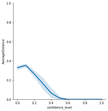
Now, we may ask a simple question: what is the effect of increasing the confidence level in the bounded confidence model? The confidence level is the proportion of dissimilarity that a receiving agent accepts from a sending agent in order for him to be influenced by the sending agent.
To answer that question, we can run the same model in the Experiment
function. Instead of a float, we pass a list of floats to the
confidence_level parameter. To get a robust estimate of the typical
outcome at each setting, we replicate all our conditions 10 times (for
11 BC threshold values that makes 110 runs in total)
experiment = ds.Experiment(
    seed=555,                                    # seed for replicability
    attributes_initializer="random_continuous",  # continuous opinion with random start value
    dissimilarity_measure="euclidean",           # distance calculator
    topology="complete_graph",                   # graph where all agents are connected
    influence_function="bounded_confidence",     # influence until dissimilarity > confidence
    max_iterations=1000,                         # simulation stops after this # of ticks
    network_parameters={                         # dictionary with arguments for 'network_init' module
        'n':20},                                 # size of the network
    attribute_parameters={                       # dictionary with arguments for 'attribute_init' module
        'num_features':1},                       # number of opinion features agents posess
    influence_parameters={                       # dictionary with arguments for 'influence_sim' module
        'confidence_level':[x/10 for x in range(11)],   # list of BC threshold values (0.0 -> 1.0, incr=0.1)
        'convergence_rate':0.5},                 # distance the receiver moves towards the sender
    repetitions=10)                              # number of repetitions per condition

results = experiment.run()
0%| | 0/110 [00:00<?, ?it/s]
110 different parameter combinations
/usr/local/lib/python3.9/site-packages/defSim/agents_init/agents_init.py:165: UserWarning: No Numpy Generator in parameter dictionary, creating default
  warnings.warn("No Numpy Generator in parameter dictionary, creating default")
100%|██████████| 110/110 [00:35<00:00,  3.09it/s]
The experiment gave us a pandas data frame with 110 rows:
print(results)
     index   Seed  Ticks  SuccessfulInfluence        Topology   n  0        0  35342   1000                    0  complete_graph  20
1        0  45985   1000                    0  complete_graph  20
2        0  31109   1000                    0  complete_graph  20
3        0  26800   1000                    0  complete_graph  20
4        0  83560   1000                    0  complete_graph  20
..     ...    ...    ...                  ...             ...  ..
105      0  75306   1000                 1000  complete_graph  20
106      0  26744   1000                 1000  complete_graph  20
107      0  44321   1000                 1000  complete_graph  20
108      0  31496   1000                 1000  complete_graph  20
109      0  74249   1000                 1000  complete_graph  20

     num_features communication_regime  confidence_level  convergence_rate  0               1           one-to-one               0.0               0.5
1               1           one-to-one               0.0               0.5
2               1           one-to-one               0.0               0.5
3               1           one-to-one               0.0               0.5
4               1           one-to-one               0.0               0.5
..            ...                  ...               ...               ...
105             1           one-to-one               1.0               0.5
106             1           one-to-one               1.0               0.5
107             1           one-to-one               1.0               0.5
108             1           one-to-one               1.0               0.5
109             1           one-to-one               1.0               0.5

      seed np_random_generator  Regions  Zones  Homogeneity  AverageDistance  0    35342    Generator(PCG64)       20      1         0.05     3.162482e-01
1    45985    Generator(PCG64)       20      1         0.05     3.381264e-01
2    31109    Generator(PCG64)       20      1         0.05     3.239260e-01
3    26800    Generator(PCG64)       20      1         0.05     3.579149e-01
4    83560    Generator(PCG64)       20      1         0.05     2.987322e-01
..     ...                 ...      ...    ...          ...              ...
105  75306    Generator(PCG64)       20      1         0.05     2.157184e-08
106  26744    Generator(PCG64)       20      1         0.05     7.696255e-09
107  44321    Generator(PCG64)       20      1         0.05     9.459349e-08
108  31496    Generator(PCG64)       20      1         0.05     3.888918e-09
109  74249    Generator(PCG64)       20      1         0.05     9.271612e-08

     AverageOpinionf01
0             0.549963
1             0.604544
2             0.441872
3             0.433244
4             0.543781
..                 ...
105           0.529282
106           0.615500
107           0.578355
108           0.375521
109           0.472806

[110 rows x 17 columns]
Using the plotting functionality in defSim (see here), we can quickly create a plot that shows the relationship between confidence level and the average distance in the plot.
plot = ds.RelPlot(ylim=[0,1])
plot.plot(data=results,x='confidence_level',y="AverageDistance")
2. Modular use
defSim consists of six different modules. Some modules take care of
model initialization (network_init & agents_init), while other
modules are called sequentially in a loop (focal_agent_sim,
neighbor_selector_sim & influence_sim), until some convergence
criterium is satisfied. The process is visualized in the flow chart
right of this text.
The Simulation class (or its wrapper the Experiment class) calls all of these modules in the background, but defSim is designed in such a way that a modular use of the package is easy and user-friendly. All modules take a NetworkX object as in- and output. Writing an extension is easy, since we can just use this networkx object to manipulate outside of one of the modules. The best way to extend the functionality of defSim is to write your extension within the defSim framework. Adding your own (published) extension to the defSim package is a great way to transparently share your code and attract attention to your work.
Now, let’s turn to two of these examples. One in which we manipulate the networkx object, and one in which we write our own module-method.
Example | Writing your own module implementation | Two groups attribute initializer
The true power of defSim becomes clear when we use custom module
implementations within the defSim framework. All calls to realizations
of a certain module in the Simulation and Experiment classes can
be replaced with your own implementation of such a module. To
succesfully pass an implementation, we need to inherit from the abstract
base classes of that particular module.
Let’s show what we mean here with an example.
Say you want to model two groups that each have a different bias in their opinions at the start of the model. Under what conditions will these two groups still converge on one position? How quick do they converge relative to if there weren’t any groups? To answer these questions we need to code an attribute initializer that will be called only at the start of the simulation.
We create an attribute initializer called MyOwnAI for ‘my own
attribute initializer’:
class MyOwnAI(ds.AttributesInitializer):
    """
    This attribute initializer creates a group attribute and assigns one of two values (0 / 1) to an agent
    with equal probability. Thereafter, the values for the `num_features' desired features is drawn from a uniform
    distribution. Limits of the uniform distribution are set for each group.
    """

    def __init__(self, limits_0 = [0, 1], limits_1 = [0,1]):
        self.limits_0 = limits_0
        self.limits_1 = limits_1

    def initialize_attributes(self, network, **kwargs):
        ds.set_categorical_attribute(network, 'group', [0, 1])
        for j in range(kwargs.get('num_features', 1)):
            for i in network.nodes():
                if network.nodes[i]['group'] == 0:
                    network.nodes[i]['f{:02d}'.format(j+1)] = np.random.uniform(self.limits_0[0], self.limits_0[1])
                else:
                    network.nodes[i]['f{:02d}'.format(j+1)] = np.random.uniform(self.limits_1[0], self.limits_1[1])
The arguments that are unique to this attribute initializer have to be
set in the __init__() part of the class. Here, we have specified
defaults for the opinion limits of the two groups ([0,1]), but these
defaults can be overwritten when we call the module later.
The initialize_attributes part of the code is simple. We set a
categorical attribute (group) randomly, and then initialize a random
opionion from a uniform distribution with limits limits_0 and
limits_1.
The new attribute initializer can now be passed to the Simulation class:
simobj = ds.Simulation(
    seed = 1414,
    topology = 'complete_graph',
    attributes_initializer = MyOwnAI(limits_0 = [0, 0.7], limits_1 = [0.3, 1]),  # here is our implementation
    influence_function = 'bounded_confidence',
    influenceable_attributes = ['f01'],         # important: only f01 can be influenced, not 'group'!
    dissimilarity_measure = 'euclidean',
    max_iterations = 3000,
    output_realizations = ['Basic', ds.AttributeReporter('group')],  # basic output is asked, and we also want to get the values for group membership back (for plotting)
    tickwise = ['f01'],
    parameter_dict = {
        'n': 100,
        'num_features': 1,
        'confidence_level': 0.6,
        'convergence_rate':0.5
    }
)
results = simobj.run()   # run the model

groups = results['group']
color_values = {0: 'blue', 1: 'red'}
colors = [color_values[group] for group in groups[0]]

ds.DynamicsPlot(colors=colors, linewidth=1, ylim=[0,1]).plot(data=results, y="Tickwise_f01")
  0%|          | 0/3000 [00:00<?, ?it/s]/usr/local/lib/python3.9/site-packages/defSim/influence_sim/BoundedConfidence.py:38: UserWarning: convergence_rate not specified, using default value 0.5
  warnings.warn("convergence_rate not specified, using default value 0.5")
100%|██████████| 3000/3000 [00:03<00:00, 879.39it/s]
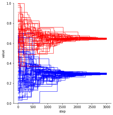
The agents neatly align into two groups. This happens based on opinion distance, but note that group membership is also taken into account when calculating distance!
Example | Independent use of modules | Biased media influence
In this example we use the modules independently. We introduce a biased media platform that will randomly influence half the population one every ten rounds. Agents follow a weighted linear influence function, which means that they are influenced proportionally to their opinion similarity to the sending agent. Once opinion distance becomes too large, influence becomes negative and agents experience a push away from the source.
Note that this could easily be done inside of the defSim framework, but we showcase here an easy to understand example of how all the modules work.
    # the INITIALIZATION stage (where the NetworkX object is set up)

# we set a random seed to be able to replicate the run
random.seed(666)
np.random.seed(666)

# initialization of the network
ABM = ds.generate_network("grid",num_agents=20)
ds.initialize_attributes(ABM, realization="random_continuous", num_features=1)

# here we introduce the biased media agent. An agent connected to all others, with a biased opinion.
agents = list(ABM.nodes())              # store the original agentset to pass to the agent selectors
ABM.add_node('biased_media')            # create new node
ABM.nodes['biased_media']['f01'] = 0.23 # fix the opinion
for i in agents:                        # add an edge between media source and all other agents
     ABM.add_edge('biased_media',i)

# initialize the dissimilarity calculator (= euclidean in the continuous opinion world)
calculator = ds.select_calculator("euclidean")
calculator.calculate_dissimilarity_networkwide(ABM)
## the SIMULATION stage (where we adjust the NetworkX object until convergence)

iterator = 0                       # to count the number of iterations
opinions_tickwise = []             # to record the opinions at each timestep

while iterator < 200:    # we stop after 200 iterations
    if iterator in [x*10 for x in range(1000)]:    # once every 10 rounds we exert media influence
        ds.spread_influence(
            network = ABM,
            realization = "weighted_linear",     # strong influence between close agents, may be negative when distance is large
            agent_i = 'biased_media',            # the sending agent (i.e. media source)
            agents_j = agents,                   # receiving agents
            regime = "one-to-one",               # communication regime
            dissimilarity_measure = calculator,  # dissimilarity calculator defined above
            homophily=1.5)                       # parameter for the 'weighted_linear' influence module
    else:                          # interaction between agents
        agent_i = ds.select_focal_agent(
            network = ABM,
            realization = "random", # select random agent
            agents=agents)          # agentset to select from
        agent_j = ds.select_neighbors(
            network = ABM,
            realization = "random", # select random neighbor
            focal_agent = agent_i,  # agent who's neighbors are eligible for selection
            regime = "one-to-one")  # communication regime, needed here to tell the selector how many agents to select
        if agent_j == ['biased_media']:        # what if the selected neighbor is the media source?
            while agent_j == ['biased_media']: # select again if this is the case
                agent_j = ds.select_neighbors(
                    network = ABM,
                    realization = "random",
                    focal_agent = agent_i,
                    regime = "one-to-one")
        ds.spread_influence(        # exert influence
            network = ABM,
            realization = "weighted_linear",     # strong influence between close agents, may be negative when distance is large
            agent_i = agent_i,                   # the sending agent (i.e. media source)
            agents_j = agent_j,                  # receiving agents
            regime = "one-to-one",               # communication regime
            dissimilarity_measure = calculator,  # dissimilarity calculator defined above
            homophily=1.5)                       # parameter for the 'weighted_linear' influence module
    opinions_tickwise.append(list(nx.get_node_attributes(ABM,'f01').values()))  # store results
    iterator += 1                  # increase iterator
The generated output is stored in opinions_tickwise – a list of
lists with all agent opinions at each timestep.
We can plot the opinion trajectories using the DynamicsPlot function
from defSim. This function normally takes a pandas data frame with a
column Tickwise_fXX generated by the tickwise output option in
the Simulation or Experiment class. If we pass a data frame with the
opinions_tickwise to the DynamicsPlot function, we can get the same
functionality:
plot = ds.DynamicsPlot(fast=True)
plot.plot(data=pd.DataFrame({'Tickwise_f01':[opinions_tickwise]}), y='Tickwise_f01')
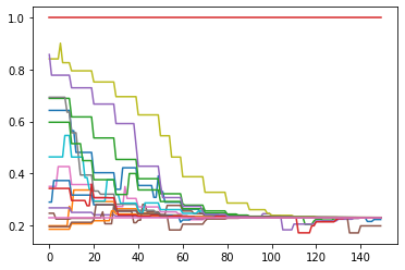
There are a few things to note from these opinion trajectories. As one might expect, a large number of the agents (90%) converge on the opinion position of the biased media source. However, in the process, two agents rejected the stance of the medium and extremized into the other direction. Occassional meeting with the other agents furthermore create temporary extremization by others, which is again corrected by the media source. To compare, let’s look at a single run of the same model without the media source.
    # the INITIALIZATION stage (where the NetworkX object is set up)

# we set a random seed to be able to replicate the run
random.seed(14)
np.random.seed(14)

# initialization of the network
ABM = ds.generate_network("grid",num_agents=20)
ds.initialize_attributes(ABM, realization="random_continuous", num_features=1)

# initialize the dissimilarity calculator (= euclidean in the continuous opinion world)
calculator = ds.select_calculator("euclidean")
calculator.calculate_dissimilarity_networkwide(ABM)
## the SIMULATION stage (where we adjust the NetworkX object until convergence)

iterator = 0                       # to count the number of iterations
opinions_tickwise = []             # to record the opinions at each timestep

while iterator < 200:    # we stop after 200 iterations
    agent_i = ds.select_focal_agent(
        network = ABM,
        realization = "random", # select random agent
        agents=agents)          # agentset to select from
    agent_j = ds.select_neighbors(
        network = ABM,
        realization = "random", # select random neighbor
        focal_agent = agent_i,  # agent who's neighbors are eligible for selection
        regime = "one-to-one")  # communication regime, needed here to tell the selector how many agents to select
    ds.spread_influence(        # exert influence
        network = ABM,
        realization = "weighted_linear",     # strong influence between close agents, may be negative when distance is large
        agent_i = agent_i,                   # the sending agent
        agents_j = agent_j,                  # receiving agent
        regime = "one-to-one",               # communication regime
        dissimilarity_measure = calculator,  # dissimilarity calculator defined above
        homophily=1.5)                       # parameter for the 'weighted_linear' influence module
    opinions_tickwise.append(list(nx.get_node_attributes(ABM,'f01').values()))  # store results
    iterator += 1                  # increase iterator
plot = ds.DynamicsPlot(fast=True)
plot.plot(data=pd.DataFrame({'Tickwise_f01':[opinions_tickwise]}), y='Tickwise_f01')
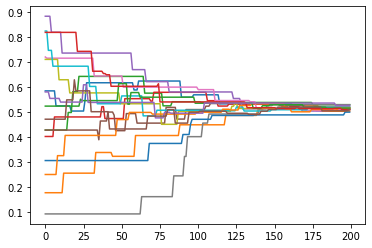
In this example the agents neatly converge to a central position